


Ore Processing Study on Copper from Scratch
- Umut Eren Yıldız

- Jun 24, 2024
- 19 min read
Updated: Jun 25, 2024
Introduction
This personal study is done for a specific report.
The personal study that I conducted was a mineral processing study. The sample was a copper sample mainly, and I focused on gaining the copper. It came from Artvin, Turkey and coded as AYE sample relatively where it is originated. I practiced a froth flotation experiment. The experiment was the 27th experiment of the same sample. The process of the experiment was lined up as at the below;
1- Sampling stage of the pre-crushed copper sample,
2- The screening process for the grinding in the rod mill,
3- Grinding stage of the sample in the rod mill before the flotation,
4- Froth flotation process,
5- Dewatering process,
6- Drying process,
7- Grade analysis with the Handheld XRF.
The Aim of the Personal Study
Firstly, the project that I wanted to conduct in this study was a flotation process. I had many chances to see the procedure in other experiments. Due to working in a mineral processing laboratory, I had to carry out a beneficiation project. I chose the froth flotation method because it is a complex operation and the most used beneficiation method in the industry.
I had a chance to work with Mr.Altun in this study. He was the director of this sample’s beneficiation project. Hence, while I was conducting the experiment, I consulted him many times, and he was so helpful. The name of the project’s sample which he was working on was “AYE”. Its initials represent where the sample came from, but the information in my report due to the institution’s policy. AYE was a copper (Cu) sample mainly because the beneficiation was focused on gaining copper. The sample contained many diverse minerals, including lead (Pb) and zinc (Zn) which mostly they are present with copper in nature. On the other hand, I was focused on copper in this study at Mr.Altun’s request, so I made my calculations on copper.
The study’s main objectives were; being familiar with the flotation process, learning how to use flotation machines and equipments, making the necessary calculations in practice, and enriching the copper as a result of the study.
Data Acquisition
The experiment that conducted by me was the 27th experiment of that project. Since it was the 27th experiment, the duration of the conditioning of the flotation experiment was determined already by Mr.Altun by the trial and error method. Therefore, I directly acquired the conditioning durations and carried out the process according to that data — the type of the data was an excel file. In addition, in the institution, engineers review the literature many times before the experiment and acquire the data and information of the past experiments on that mineral.
Grinding tests were required for all the grain sizes that we were working with because of finding the optimum size to work with on flotation.
Analyses and Calculations
I would like to examine this study part by part. There were five main stages for the study; sampling and weighing processes, sieve test analysis after sampling process, grinding in the rod mill and cleaning the rods processes, flotation process, drying the sample in the furnace after flotation, and preparing the sample for grade analysis.
Sampling and Weighing Processes
First of all, the AYE Sample was already pre-crushed and ground to -38 µm. Mr.Altun brought a 10,560 g AYE sample, which is weighted. The next stage was sampling. Sampling is needed for the beneficiation process because when the sample is subjected to flotation and analysis after flotation, it should be homogeneous to get the most precise results.
Chute Riffler is used for the first sampling stage. Chute Riffler is an equipment that divides the feed into two samples.

Firstly, the sample is fed the inlet of the chute riffler and divided into two identical samples, which were A and B. Then, both of them were divided into two more samples. Hence, four identical samples were acquired (C, D, E, and F). After that, for creating more homogeneous samples, C and E were combined, and D and F were combined. They were subjected to one more division, so the same procedure was done. At the final, four identical samples were obtained. In addition, they were named as G, H, J, and K. The organization charts that represent the procedure are at the below.


To see the difference from average weight, some calculations are made, and a table is prepared. The created table and some example calculations are at the below.

Whole sample = 2613 g + 2632 g + 2671 g + 2644 g = 10560 g
10560/4 = 2640 g
For G →(2640 * 100)/ 2582 =102.24, 102.24–100 = 2.24 %
For H→ (2663 * 100)/ 2640 = 100.87, 100.87–100 = 0.87 %
For J →(2713 * 100)/2640 = 102.76, 102.76–100 = 2.76 %
For K →(2640 * 100)/ 2602 = 101.46, 101.46–100 = 1.46 %
According to the lab manual (Chapter 1 — Sampling, n.d.), the standard deviation of the samples is 1.01 in theory if the Chute Riffler is used and the experimental standard deviation that was found is 0.72. Hence, the sampling is considered as successful.
Second Sampling Stage
The first sampling process was done. Before weighing the samples for the flotation process, another sampling operation had been seen as necessary.
For the second sampling stage, a small spinning riffler is used. The equipment was using the centrifugal force to distribute the samples into the bottles, of which there were eight of them. The inlet part was at the top. Samples fell into the channel, which was vibrating to convey the particles from the inlet. Then, they were separated into eight bottles by centrifugal force. In addition, some particles were stuck on the pipes of the bottles, at the inlet or at the bottles inlet. Hence, the Allen key was used to give a better vibration while the riffle was spinning. The figure of the procedure is at the below.

Every sample (G, H, J, and K) was fed separately. Samples were meant to be packed as 1000 grams per one. Each bottle contained nearly 325 grams. Therefore, every package included three bottles. After completing every package, they were rounded to 1000 grams with the remaining single bottles. In addition, bottles were selected diagonally for the samples separately. In the end, samples were arranged as 1000 grams, and ten-piece of the sample was prepared. The leftover nearly 500 grams was considered as waste.


Sieve Test Analysis After Sampling Process
A sieve test is required to determine the range of the particles and the amount of them in each size. A sieve test analysis is a screening procedure on a laboratory scale. The main reason for the screening is to see the fractions to determine if another size reduction is necessary or not. In addition, after screening, the cumulative undersize graphs can be created to find the size, which is important to make some calculations in industrial-scale works.
Screening can be operated dry or wet. The advantage of wet screening is that washing down the particles is more effective than dry screening if ore does not have a tendency to be slime. For the experiment, by the suggestion of Mr.Altun, the dry sieving was done firstly to see the fractions sketchy. Ro-Tap Testing Sieve Shaker was used in 1000 rev/min for 10 minutes for the dry sieving.

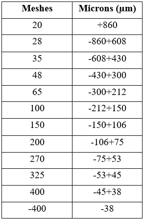
Both for the dry sieving and wet sieving, the same sieves were used. The sieves were chosen according to (2^0.5) rule. Starting with 38 microns, sieves were multiplied by (2^0.5)each time and meshes were determined as in the figure.

After a sketchy dry sieving, wet sieving operation was started. Due to equipment errors possibilities, sieves were not cumulated on another. They were placed, and they screened one by one. The first sieve was the +20 mesh to screen the coarser particles, and the procedure went through as in the figure.

Oversize material was cumulated on the sieve, and undersize material was washed down the sieve into the bucket with the water. The machine was stopped, the sieve was taken, and oversize material was washed with a pisset into a tray, then, same procedure into a beaker from the tray. After that, waited for the precipitation of material and drained slowly. The sample was ready to put into the furnace for drying.

While this procedure was kept going, the undersize material was precipitating. It is also drained because of lessening the circulating load of water. Then, the undersize material in the bucket was used for the feed of the next sieve, as in figure. The same procedure was repeated for all the sieves.

After applying the same process for all sieves, samples were ready as fractions and were put in the furnace for drying for 24 hours.

As the last for the sieve test analysis, equipments were cleaned up. Especially sieves were placed in the ultrasonic sieve cleaner, which cleans the openings from the stuck particles with ultrasonic sounds.

Results and Calculations
After 24 hours, dry samples were weighted for each fraction, and a table was generated as in figure.

As said before, one of the main reasons for the sieve test analysis is finding the value. Hence, after reaching the cumulative undersize material in percentage, a graph can be created, which is named as Tromp Curve. X-axes represent the particle size in microns, and Y axes represent the cumulative undersize material in percentage.

The value of can be found by implementing a power trendline to the curve. From the curve, the equation can be obtained. Following calculations are made to find the size of the sample.
For finding the size of the particles, 80 is placed to y in the equation to find the x.

While the y is equal to 80, µ is equal to 447.1 µm.
In addition, to see the distribution of the oversize material, a distribution graph can be generated.

The Imperfection Value is a parameter that is calculated for determining how sharp the separation. Following calculations are made to find the Imperfection Value of the separation.
For finding the imperfection value;

Grinding in the Rod Mill and Cleaning the Rods Processes
Comminution is a significant operation. It mainly prepares the ore for the selected beneficiation method on a laboratory scale. In the flotation experiment cases like this experiment, an optimum size is required for floating the particles. If particles are bigger than they should be, gravitational force dominates the adhesion force between the bubble-particle, bubbles will not be able to carry, and bubble-particle attachment can not be maintained, so they do not float. If they are too small, they will not attach to bubbles.

The experiment that I was conducting as a personal study was the 27th experiment, as mentioned before. Hence, the grinding tests for the ore to determine the duration of grinding were already calculated. At Mr.Altun’s request, the grinding test was counted as valid for this experiment too.
The grinding tests are simply conducted by trial and error method. Samples were ground for 10 minutes, 20 minutes, 30 minutes, and 40 minutes with a determined rpm number which is 44 rpm. Then, each time they were subjected to sieve test analysis, and cumulative undersize material was determined.

After obtaining the values as in the table, a graph was generated. In the graph, X-axes represent the grinding duration, and Y-axes represent the cumulative undersize material. A line is created for every particle size on top of each other. Then, a vertical line is pulled to the X-axes from the horizontal d80 cut size. Thirty-three minutes was determined, which corresponds to 38 microns because we were working with the 38 microns as the smallest particle cut size.


Later calculating the duration of the grinding, the rpm calculations are required. There are certain equations for both the rod mills and ball mills to calculate the interval of grinding rpm.

After wet grinding the sample with 44 rpm for 33 minutes, the sample was slowly poured into the flotation cell, as shown in figure. Then, inside the mill was washed with the washing bottle into that cell to not leave any particles in the mill. Also, the same procedure was applied to the rods as in the figure.


Flotation Process
Flotation is a process that benefits from the differency of physicochemical properties of minerals according to lecture notes of METU (Chapter 10 — Froth Flotation, n.d.). It is one of the most used methods in the mineral processing work field. The main purpose is to make the particles hydrophobic to float them. Hydrophilic particles precipitate at the bottom, and hydrophobic ones float. There are reagents for conditioning the pulp.
Firstly, the experiment was done with the same sample. Hence, some of the parameters were already decided by Mr.Altun. According to Mr.Altun, parameters as the duration of conditionings after adding reagents, durations of skimming the froth, pH needed for the flotation of mineral (determined by the zeta potential studies), and amount of the reagents were determined by the error and trial method. He had done literature research such as how much pH was needed to conduct experiment or which reagents were used for the copper mineral in the past experiments. So, after deciding the reagents, he had changed a parameter for each experiment at a time. For example, he had kept constant the concentration of the MIBC and had changed the conditioning duration of MIBC. Then, when the conditioning duration was determined, he had tried to determine the concentration of the MIBC. Hence, he had stated the optimal parameters.
The experiment that was conducted by me was a direct flotation process in which the valuable mineral was floated only and consisted of three procedures: rougher cell, cleaning cell 1, and cleaning cell 2. There was no scavenger cell. So, at the end of the process, four products were reached. The circuit’s schema of the procedure is shown at the figure.

After grinding, the cell was placed under the flotation machine. Conditioner was opened to make the pulp homogeneous, and a pH meter was placed in the flotation cell. pH was important for the experiment because of the flotation of copper, the pH of the environment should be at least 11.5. Arranging the pH of the pulp was controlled by slaked lime (Ca(OH2) ). The flotation machine was operated at 1450 rpm. After arranging the pH, fifteen minutes were waited for conditioning. Then, KEX was added to the pulp as a collector, and waited for conditioning five minutes. The collector made the copper minerals gather together at the surface. MIBC was poured into the cell and waited again for one minute. MIBC was acted as a frother and helped the froth of the copper on the surface and prevent the froth breakage, according to METU mine310 lecture notes (2021).


The air valve was opened, and the air started to get in from the inlet to create the bubbles at the surface, bubbles started to gather — hydrophobic copper particles attached to the bubbles on the surface. Froth was skimmed for 10 minutes. The rougher flotation process was completed after skimming the froth. General data is given below in the figure.


After the rougher cell was skimmed. There were two products; the concentrate, which was the froth, and the tailings, which was the sink. At the rougher cell, most of the silicates were removed as tailings. So, when the concentrate of the rougher cell was subjected to cleaning, flotation had been more efficient.
The tailings of the rougher cell were transferred to the filtering machine. Stuck particles were washed by the pisset water, and the machine was closed. Then, the pressure was opened, and water started to drain. After water stopped coming, the machine was opened, and the sample was taken. The pressure filtering machine dewatered the sample for preparing it for the drying process, and it is shown in figure.

The cleaning cell procedure was started with the concentrate of the rougher cell. Revolution per minute was dropped to 1000 rpm, and skimming duration was decreased to 5 minutes after pH conditioning for 5 minutes. At the skimming step, it was clear that silicates were removed at the rougher cell because the copper color and particles were much more clean and dominant at the froth.

After the first cleaning, filtering was applied to tailings of the cleaning cell as like the tailings of the rougher cell. The concentrate was taken to another cleaning procedure with the same conditions as in the figure.

When the second cleaning cell was completed, tailings and concentrate of the second cleaning were dewatered. The concentrate of the second cleaning was the ultimate concentrate. Hence, the four filtered products were achieved, which were DS-K, DS T1-A, DS T2-A, DS-A. After the samples were filtered, they became a filtered cake layer.

Drying the Sample in the Furnace After Flotation and Preparing the Sample for Grade Analysis
The drying process is the last stage for the ore preparation before the grade analysis in the laboratory. After the filtration of the sample products DS-K, DS T1-A, DS T2-A, DS-A, they were placed in the furnace for drying. They could not be weighted as wet because it would not give the correct weight distribution results. Sample products were stayed in the furnace for 24 hours.

Then, samples were took and controlled if they were dry enough. After deciding that they were dry, they were scratched out from the filter paper with the spatulas and crumbled by hand.
Every crumbled sample was weighted on the precision scale and recorded. The weights of every product are shown at the below figure.

The input feed of the sample that entered the circuit was 1000,5 grams. The output feed was calculated as 1003,95. The main reason for the weight increase is the addition of slaked lime during the flotation for arranging pH.
The samples were packed in small sample bags, and their names were written on the bags. Hence, they were ready for the grade analysis.

Analyses By The Experimenter With XRF
After finishing the experiment and preparing the samples, a grade analysis is required because the company that is excavating and extracting the minerals determines the amount of beneficiation cost on an industrial scale and how much ore that is aimed to gain in the samples for the earnings. In addition, the efficiency of the samples is beneficial for the company if the ore is worth extraction, which can be calculated from the grade values.
For this experiment, instead of the laboratory analysis, handheld XRF machine was used. XRF machines are not precise mostly. Although, according to Mr.Şen. Hence, the values must be strongly close.

A little amount was taken from each sample (DS-K, DS-A, DS T1-A, DS T2-A) and arranged in a small box. Then, they are placed in the XRF cabinet one by one and subjected to test. Handheld XRF inspects the mineral grades by using the X-Ray Fluorescent.

The following figures show the grades of the concentrate, middling 1, middling 2, and tailings.


Note: The values shown without the percentage marks are in the ppm content.
After the analysis, a grade distribution and efficiency table can be generated. The table is shown at the below figure.

Results and Conclusions of the Personal Study
A flotation experiment is one of the most used methods due to its low OPEX (operational cost). In addition, it is a resourceful method compared to other methods. In this experiment, I conducted a froth flotation experiment and supervised by the engineer Mr.Altun. Many conclusions can be derived from the study. Hence, I would like to examine the results part by part as like the study:
1- Sampling and Weighing Processes
2- Sieve Test Analysis After Sampling Process
3- Grinding In the Rod Mill and Cleaning the Rods Processes
4- Flotation Process
5- Drying the Sample In the Furnace After Flotation and Preparing the Sample for Grade Analysis
6- Analyses By The Experimenter With XRF
1- Sampling and Weighing Processes
Sampling in the laboratory can be conducted with different kinds of equipment and methods. Some of the methods are scoop sampling, cone and quartering, chute riffler, spinning riffler, and table sampler, according to Abouzeid (1990), as mentioned in the laboratory manual.
The techniques that were used in the study were chute riffler and spinning riffler. The main reason for sampling is to obtain homogeneity. So, the separation procedure can be processed successfully.
The equipments have a separation efficiency. The numbers are generalized from the practices. According to Khan (1968), standard deviations of the sampling equipments are at the below figure.

In the study, the whole sample was 10560 grams as the amount. After the chute riffler technique, a data-sheet was prepared, and for every sample, the value of difference from average weight in percentage was calculated. The standard deviation of these values gives the method’s generalized standard deviation. The experimental standard deviation was found as 0.72, and the theoretical standard deviation is 1.01. Hence, the sampling procedure of chute riffler was considered as successful.
After the chute riffler, another sampling technique was applied; spinning riffler. A small spinning riffler is an equipment with eight bottles at the outlet of the equipment. In each bottle, there were nearly 330 grams of sample. The amount of weights in the bottles at the chute riffler was not noted for every bottle. So, the standard deviation of the process could not be calculated.

2- Sieve Test Analysis After Sampling Process
Sieve test is a screening method. Screening is important because the d80 cut size of the sample is found by screening.
The experiment was conducted dry at first. The main purpose of doing that was to see the fractions roughly which were seen. Although, it was not the whole process of screening. Then, the wet screening process was applied, which was the final separation method. According to Mr.Altun, wet separation was more efficient because the mineral was not turning into a slurry with the water due to characteristics, and the pressure force that comes with the water washes down the particles from the apertures especially the ones which causes screen blinding.
On the other hand, undersize particles were washed down into a bucket after the sieving from each sieve. Hence, a pulp was generated in the bucket. The pulp was waited for decantation to take place. Then the draining was performed to not to add more water to the circulating load.
In the figure, some calculations were made to generate the table. For example, calculations are shown at the below.
After the mesh number’s and aperture size’s values were entered, the weights of the retained on each sieve were written. Then the percentage of the weight was calculated as;

Then, the cumulative weight retained on the sieve (%) was calculated by adding the percent weights going downwards as cumulative.

The cumulative weight passing the sieve was found by subtracting the oversize (%) material from the whole sample (100%). It is calculated as;

Hence, the table was generated to make the necessary calculations.
After creating the sieve test analysis table, a tromp and a distribution curve were generated to observe the separation’s efficiency and find the required cut sizes. In the figure, the distribution curve of the screening was shown. The X-axis represents the particle size in microns, and Y-axis represents the oversize material on the sieve as a percentage. At the end of the curve, there is an instant fall in the values retained on the sieve. That was caused by the over-grinding. Overground material was passed from the +20 mesh sieve easily. On the other hand, the fluctuation at the middle between 75 and 212 microns was not normal, and that shows the sieving between the +200 and +65 meshes sieves was not efficient enough. Hence, the screening was not optimal and successful.
The imperfection value is a parameter for determining the efficiency of the separation. The imperfection value is found by determining the d75, d25, and d50 cut sizes from the tromp (partition) curve. The general formula of the imperfection value is

The calculations showed that the imperfection value is 2.62. According to Heiskanen (1993), the imperfection value should be between the values 0.22< I < 0.71 to be accurate. Hence, the number 2.62 shows that the sharpness of the separation was not reasonably required.
3- Grinding In the Rod Mill and Cleaning the Rods Processes
Grinding is an important process to prepare a sample for the beneficiation method, and it is the last stage of comminution. In the experiment, the grinding process was done in the rod mill with different sizes of rods which the biggest one has 3.3 cm diameter.
After grinding in the mill, the direction of the inlet of the equipment was slowly changed downward, and the sample was taken as pulp to a flotation cell. Then, the rods were washed with a pisset as mentioned as like inside the mill. The main reason for washing was to leave no particles in the mill. Because, according to Mr.Şen, even if less material was left stuck to particles, the experiment should be counted as invalid. Every weighed particle has value.
In the figure, the undersize material versus grinding duration graph is shown. The X-axis of the graph represents the grinding durations in minutes, and Y-axis represents the undersize material in percentage. The graph was generated after grinding the sample for 10 minutes, 20 minutes, 30 minutes, and 40 minutes. Each time after grinding, the sample was subjected to screening with the wet sieve test, and the figure. was generated. The graph was created according to the table. Each line represents a different cut size of the sample. To reach the accurate grinding duration, d80 cut size of the 38 microns were chosen, which corresponded to 33 minutes.
For the grinding process, equipment was run at 44 rpm. According to engineers, the rpm number was calculated by the firm that supplied the equipment, and it was constant. Although, I calculated the critical speed of the mill with the critical speed formula with respect to lecture notes (n.d). According to the results, the % critical speed was calculated and found as %40.55. According to lecture notes, the tumbling mills are driven at 50–90% of the critical speed. At the lower speeds of this interval, cascading movements dominate the motion, and at the relatively higher speeds, cataracting movement dominates. Hence, the rpm number that was worked with was relatively low than it should be. Cascading movement leads to finer particles that become slime and can not float easily.
4- Flotation Process
At the flotation process, to increase the pH, slaked lime was used, which is a basic chemical. Slaked lime (calcium hydroxide) can be produced from the lime (calcium oxide). The relative equations are at the below.

When the calcium hydroxide is dissociated in the water, it breaks into ions, and this reaction brings the basic characteristic into the environment by the hydroxide.

Moreover, MIBC (frother) was newly prepared before the experiment. Hence, during the skimming process, the pulp was froth greatly, which affected the concentrate’s grade.
Silicates were tried to remove during the rougher cell. The main reason for this is to increase the efficiency of the concentrate in the rougher cell. On the other hand, at the cleaning cells, rising the grade was the main purpose for a more pure copper concentrate.
5- Drying the Sample In the Furnace After Flotation and Preparing the Sample for Grade Analysis
Drying is an important process because the actual amount of the samples can be obtained after drying. The dewatering procedure can filter the sample after flotation, but the sample would be still moist, so drying with the heat and oxygen in the furnace can only determine the real amount of the samples
6- Analyses By The Experimenter With XRF
The handheld XRF is equipment that can be seen rarely in Turkey, according to Mr.Şen. On the other hand, many companies have handheld XRF, but they can only read metallic minerals. The machine uses x-rays to detect the minerals in the sample and shows the content of the sample nearly in a minute.
In the figure, the distribution of the grade and efficiency is shown. The general efficiency can be calculated by subtracting the tailings’ efficiency from the whole. It is demonstrated at the below.

If there is a comparison of the efficiencies between the past experiments and the DS experiment, the efficiency of the concentrate in the DS experiment is much higher. According to Mr.Altun, that might be caused by the frother because the MIBC was newly prepared and undecayed. Hence, it worked much better. As can be seen from figure, the main Cu content came to the concentrate from the middlings, especially from the middling 2.

In general, the experiment was successful. Copper concentrate was taken as the grade in 90,97%.

I learned from the grinding process that equipment should be washed into the cell very carefully to get better efficiency.
CONCLUSIONS
In a nutshell, working with the engineers was a very eye-opening experience. Everyone in the company was very helpful, understanding, and welcoming. The knowledge that I have acquired in the class was turned into practice. I have experienced the working environment. With that, I learned the time-management of every stage of a beneficiation experiment. I had a chance to get to know the departments and working styles of the company.
By conducting my experiment, I got familiar with all the stages of flotation. In addition, working on a schedule made me more programmed and a more efficient worker.
I can say that working in a mineral processing department and being able to use all the laboratories that include any beneficiation equipment is very beneficial. Doing many experiments and trying to reach the most effective result can show the person every possible sight of error and accomplishment, and to me, that is a great experience.


Comments